IMP: CoordGen8- Coordinate Generation Utility: User’s Manual
H.David Sheets, Dept. of Physics, Canisius College, 2001 Main St.,
Buffalo, NY 14208. sheets@canisius.edu.
The IMP software series is a set of tools for the analysis of biological shape using landmark-based morphometric geometric methods, and CoordGen7 (COORDinate GENerater) is a software tool for generating various superimpositions of the landmark configurations. CoordGen7 can generate, display and save data sets in Partial Procrustes Superimpositioning, Bookstein Coordinates, Sliding Baseline Registration and RFTRA superimpositioning. The input files needed for CoordGen7 may be in TPS file format (F.J. Rohlf, 1993-present, see the morphometrics web site at SUNY Stony Brook, http://life.bio.sunysb.edu/morph/) as produced by the TPSDig program (Rohlf, 1998), or in the x1y1x2y2...CS file form used by IMP, in which each specimen is arrayed on a row of a matrix (see further discussion below), or in the MorphoJ format (Chris Klingenberg, http://www.flywings.org.uk/MorphoJ_page.htm) which is a text file with specimen labels on each line and a header. The output files are in any of these three formats.
Additionally, CoordGen can rescale the data using the endpoints of a ruler included in the measurements of landmark locations, display the landmark configurations in each of the superimpositions, and generate reference forms from the data in each superimposition. There are also tools meant to look for errors in digitization (including a simple PCA plot, and an approach to determining which landmarks make large contributions to the total variance), to calculate variance in shape and in centroid size, as well as to work with data in the Procrustes Size Preserving (Procruste SP) superimposition. The program can compute and export the variance-covariance matrix of all specimens and the matrix of pairwise Procrustes distance between all specimens, which may be useful in other programs. This version of CoordGen will incorporates the older IMP TradMorphGen program for calculating lengths between landmarks and angles and also the SemiLand program for carrying out semi-landmark analysis.
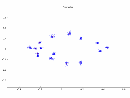
The image
above shows 16 landmark coordinate measurements from 46 specimens of Serralmus
elongatus (a piranha) in a Partial Procrustes Superimposition (CS=1)
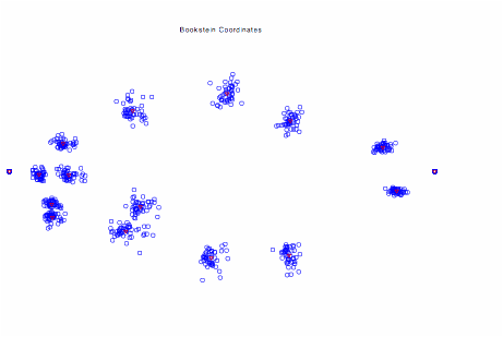
The image
above shows 16 landmark coordinate measurements from 46 specimens of Serralmus
elongatus (a piranha) in Bookstein Coordinates (registration to a baseline).
CoordGen7 forms the “entry-point” to the rest of the tools in the IMP series. All other software tools in IMP use the same file format, and this file format also loads directly into Excel, SPSS, SAS and other software packages, since the data are stored in a data matrix such that each row is a specimen, and each column is a coordinate. The MorphoJ file format may also be helpful when exporting data into other software packages, as it includes a header line and specimen labels.
This manual will not serve as an introduction to Geometric Morphometrics, if you are completely new to the field, spend some time browsing the website at StonyBrook run by F. James Rohlf (, http://life.bio.sunysb.edu/morph/) or the reference list at the end of this document to locate further resources.
Credits:
Conceptualization and GUI Design: H. D. Sheets, D.L. Swiderski, M.L. Zelditch
Coding and Software Design:
H. .D. Sheets -sheets@canisius.edu, Dept. of Physics, Canisius College, 2001 Main St. Buffalo, NY 14208, 716-888-2587
Referencing:
The IMP series is completely free, but I would appreciate being referenced if you use it in published work.
Please reference my name and address, and ideally the website address,
http://www.canisius.edu/~sheets/morphsoft.html
or
the textbook, Geometric Morphometrics: A primer. Zelditch M.L., Swiderski D.L., Sheets H.D. and
Fink W.L. 2004. Elsevier. (2nd edition under contract, scheduled for
completion January 2012).
Topics Covered in this Manual
Input
File Formats (IMP, tps, MorphoJ)
Loading
and Saving Data
Output
File Formats
Detecting
Digitizing Errors
Detecting
Noisy or Difficult to Digitize Landmarks
Variance
Procrustes
SP results
Summary
Information about Data sets
Calling
Other Tools
TMORPHGen
SemiLand
Miscellaneous
Buttons and Commands
Using
CoordGen7
CoordGen7 is a Coordinate Generating program meant to generate data files of landmark based geometric morphometric data in different types of superimpositions, Bookstein Coordinates (BC), Sliding Baseline Registration (SBR), Procrustes Superpositioning (PS) and Resistant Fitting Theta Rho Analysis (RFTRA). The program also displays data sets and allows for the generation of mean or reference specimens in each type of superimposition. The output files can be generated in the TPS format used by James Rohlf's software or the x1y1x2y...CS format favored by Zelditch, Sheets et al, and the MorphoJ format used by Chris Klingenberg. The program will also compute summary statistics for the data set, and has tools meant to allow detection of digitization errors. It will also save matrices of all inter-specimen distances.
Input File Formats
The program can currently load three distinct data types,
TPS files
This is the file format used by the
tps software series, including the extremely useful
tpsDig tool for digitizing images. The
following tps file variants can be loaded into
CoordGen, Landmark data
-with a ruler visible in the image,
-with no ruler, but already properly scaled
-with a scaling factor for each specimen.
-with curves which will be converted into semi-landmarks
-with curves and a ruler
X1Y1 formats
These are input files with one specimen per line, with each column being a variable (landmark coordinate). The first column is the x coordinate of the first landmark, the second column is the y coordinate of the 1st landmark, followed by the (x,y) pair for each consecutive landmark. The specimen name may appear at the end of a line after a percent sign (%specimen 411), see details below
-X1Y1 raw data with a ruler in the file
-X1Y1 Raw data with no ruler
-BC Files (X1Y1..CS)- this is the IMP format default file used elsewhere in IMP. The name BC refers to our early practice of saving all data in Bookstein Coordinates, with the centroid size(CS) as the last data column. If specimen labels are used, they are after a % on the last line of the file.
MorphoJ format
In the MorphoJ format, each specimen is on a single line, the first entry in each column is the specimen name, followed by each landmark coordinate in (x,y) pairs. Data is scaled to the size of the specimen.
Formatting, reformatting and viewing of data files may be done using Word or Excel, or any other program that is capable of outputting ascii text files. The 'Save As' option in Word or Excel will let you specify MS-DOS text files which work well.
Loading and Saving Data
Most load options are available using buttons on the main screen, others must be accessed through the file menu.
Loading TPS files
To load a TPS file, the TPS format rules must be followed, see the documentation with F. James Rohlf's software(see the website listed earlier, or the example below). The only critical factor for CoordGen is that the symbol sequence LM=XX be on the line immediately before the set of values representing the coordinates of each specimen, where the x and y coordinates are paired on each line. XX is the number of landmarks. Any information after the number of landmarks following LM= is ignored, so this is a good place to put a specimen label or other comments.
If you are loading a file that has a ruler in the image, the software assumes that the ruler is the last two landmarks in the list, and that the ruler has a length of 10 units. If this does not match your data, use the ruler endpoints boxes to specify where the ends of the ruler are, and the ruler length box to specify the ruler length. Then use the carry out rescaling button to re-adjust the value of the landmark positions and calculate the centroid size.
If you have no ruler in the image, CoordGen can load the data assuming it to be in properly scaled units Load tps (no ruler/no scale factor), and to need no further rescaling. It is also possible to to a tps file with a scale factor (this option is on the File menu).
When you load a tps file, CoordGen will attempt to extract some labeling information from the tps file, collecting information from three different locations in the tps file.
a.) on the LM= N line of the tps file, CoordGen will read any information following the value of N and include this information in the specimen label. If the LM line reads “LM=12 NmFaS#311.2”, then the letters “NmFaS#3112” will appear in the specimen label.
b.) if the is an ID=M line in the data file, CoordGen will append the ID number to the information on the LM= line. So if in the file above, the id line was ID=7, the “7” would be appended to the label, to read “NmFaS#3112 7”
c.) if there is a line with the image file name, IM=filename, in the tps file, CoordGen will append the image file name to the data label. If the the file discussed above has the line im=”NMFAS_3112.tif”, the entire data label would read
“NmFaS#3112 7 NMFAS_3112.tif”
This process does have the possibility of generating unwieldy specimen labels, but allows for a lot of labelling options. All IMP series programs keep specimens in the same order as they were input into the program and typically refer to specimens by their ordinal number in the file, although some functions will use the label.
Loading X1Y1 data
These are all variants on the standard IMP format, which were developed using earlier versions of Matlab. In each case, a specimen occupies one row of a data matrix, and each column is a landmark coordinate (or the centroid size). This format is easily loaded into Excel or systat.
X1Y1 Raw Data With Ruler
This file format consists of the set of landmark measurements for each specimen arranged as the row of the data matrix. The first column is the x coordinate of the first landmark, the second column is the y-coordinate of the first landmark, followed by in successive columns by the x and y coordinates of all other landmarks in order. This option again assumes that the endpoints of a ruler are included in the landmarks, the endpoints of the ruler are used to rescale the rest of the data.
X1Y1 Raw Data (no ruler)
This is identical to the format used for the X1Y1 Raw Data with Ruler as discussed above, except that there is no ruler. The data is assumed to be correctly scaled.
X1Y1...CS Files, Format and Input
In this file format (loaded using the file labeled “Load BC File (X1Y1..CS) IMP standard format”), the coordinates of all landmarks corresponding to a single specimen lie on a single row or line of the file. The X coordinate of each landmark is listed first, followed by the Y coordinate, with a space between each. The Centroid Size (CS) of the data is the last item in the list. Following centroid size there may be a percent sign (%) followed by a data label. All text and numbers following the % are treated as labels. So for data in 2 dimensions with k landmarks, there are k pairs of X Y values plus CS or 2k+1 values on a single row or line. Each line of the file is a separate specimen. All of the IMP software using this system is written to avoid changing the ordering of specimens, so that the order of all specimens in an X1Y1...CS file is fixed, and the same as the digitizing file it was created from. Most (but not all) of the IMP programs will recognize and load the data labels.
Coordgen will load X1Y1...CS files in, so that you can convert from one superposition to another, or generate reference forms or plots from it.
Sample X1Y1...CS file format
0 0 1 0 0 1 1 1 4 % sepecimen 1
This is an X1Y1 file for a square in BC with corners at (0,0), (1,0), (0,1) and (1,1) which had a centroid size of 4 before being placed in BC registration.
Output File formats (Landmark data)
The output file format button will allow you to chose the output format you want, either TPS for use with Rohlf's software or X1Y1...CS format for this software suite. You can then save using any number of different superimpositions. We have often saved data in Bookstein Coordinates (BC) when saving in IMP format, as the baseline endpoints will be at (0,0) and (1,0), making it eas to see column positions of LMs in Excel. Most IMP software allows you to specify the superimposition to use (recomputing it each time), so the superimposition you save data in is not critical when working with IMP. MorphoJ output format is also available on the file menu.
The program will output data in a variety of superimpositions when working with tps or IMP file formats. The IMP format loads easily into programs like Excell, SPSS, etc. Note that in all the IMP output formats, the last column is always the CS value. Data labels are at the end of the line, separated by a percent sign (%).
When you use the save data in MorphoJ format (using the File Menu), the data is first placed in a Procrustes Superimposition and then multiplied by the CS so all the interlandmark distances are correct. Since the centroid size of each specimen is now equal to the measured CS, these data are appropriate for use in MorphoJ, where the program will carry out a Procrustes superimposition. They are not properly scaled shape data for use elsewhere though, since the Centroid size is not one.
Other Output Files
The option to Save All Pairwise Procrustes Distances on the File menu will save a matrix of all Partial Procruste Distances between all specimens to a file. The rows and columns of this matrix correspond to the ordinal position of the specimens in the input data file. This matrix may be used as the input to a Non-metric multidimensional scaling (NMDS) program such as PAST (Hammer, 20XX) or to a Permutation MANOVA program (Anderson 200X).
Detecting Digitization
Errors
One of the common errors in
digitizing is to swap the order of two landmarks in the order of digitization,
a problem which is difficult to see in a Procrustes plot. Fortunately, errors like this are easy to
spot on a PCA plot, since this error will produce a large variance in the data,
and result in the specimen with the error being well separated from the others
on a PCA plot. CoordGen has a quick PCA
tool, which shows only the first two PCA axes scores of all specimens, with
specimens numbered on the plot, as a tool for locating digitizing errors. This tool is accessed through the “Call Other
Tools” menu. For a more complete PCA
tool, see IMP PCAGen7 or tpsRelWarp.
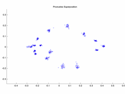
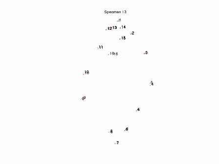
In this example data set of
landmarks on piranha, specimen 13 has reversed LM ordering. It is not particularly visible in the
Procrustes Plot of the data.
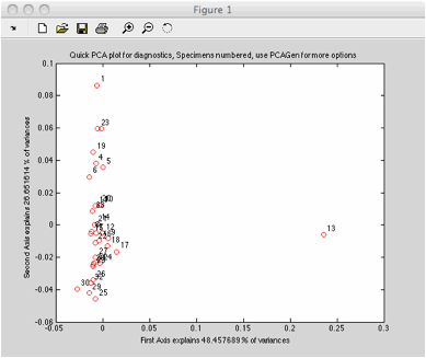
The quick pca immediately shows
specimen 13 as an outlier.
CoordGen will also display single
specimens at a time, using the show individual specimen controls. You can specify the specimen to show by
listing it’s ordinal value, and can plot it along with the mean (in Procustes
format). This is intended to allow
specimen by specimen examination of your data set.
When specimen 13 (blue) is plotted with
the mean (red), with numbered landmarks on each, it becomes clear that the
number of landmarks 4 and 5 is reversed on specimen 13 relative to the
mean. The zoom function may be necessary
to clearly see LM numbers in this view
Detecting
“Noisy” or Difficult to Digitize Landmarks
In some studies and organisms, some
landmarks may be difficult to reliably locate and digitize, relative to the
other landmarks. When working with
shape data, landmark locations are relative to all other landmarks, not absolute
or independent quantities. This makes it
a bit difficult to determine the cause of excess variation or randomness, since
variance is a property of the whole set of landmarks, not of each landmark as
an individual.
What we can do is compute the variation
in LM position around the mean shape, omitting on LM at at time in the
calculation. When we omit a landmark
that is difficult to reliably digitize, we would expect the variance around the
mean to decrease, relative to the variation seen when other landmarks are
omitted. CoordGen can do this calculate
of variance, systematically omitting landmarks, and then display a list of
variances values as shown below for the piranha example above, sorting in order
of increasing variance. This option is
available on the Call Other Tools Menu, under the LM Contributions to
Variance option.
The variation in the data set will
be reported both as a function of the omitted landmark, and in the form of a
histogram.
|
LM Omitted |
Variance |
|
4 |
0.0027743 |
|
5 |
0.0027828 |
|
10 |
0.0035901 |
|
16 |
0.00363 |
|
11 |
0.0037165 |
|
9 |
0.0037207 |
|
3 |
0.0037374 |
|
1 |
0.0037899 |
|
15 |
0.0038604 |
|
14 |
0.003873 |
|
2 |
0.0038964 |
|
13 |
0.0039513 |
|
12 |
0.0039574 |
|
6 |
0.0042497 |
|
8 |
0.0042787 |
|
7 |
0.0045109 |
|
|
|
In this example, rather than an
unreliable landmark, the position of LM 4 and 5 was swapped for specimen
13. This does appear in the listing
above as though LMs 4 and 5 were large contributors to the variance (since
variance drops drastically when they are omitted). CoordGen will also plot a histogram of the
variance values and the number of occurrences of each value, which one can use
to determine if the “noisest” landmark is really different from the other
landmarks, or part of a smooth distribution.
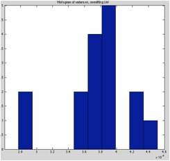 In the piranha example, the two variance
values on the left side of the plot are not part of a smooth distribution of
variance values, rather they are isolated low values, indicating these two
landmarks do not have the same distribution of error as the other landmarks
do.
In the piranha example, the two variance
values on the left side of the plot are not part of a smooth distribution of
variance values, rather they are isolated low values, indicating these two
landmarks do not have the same distribution of error as the other landmarks
do.
Evidence like this in a real study,
and not due to landmark mis-labeling, might be evidence that one or more LMs
were unusually hard to accurately digitize.
Variance
CoordGen7 will also compute variance
and RMS scatter statistics. Variance is
calculated as the summed squared procrustes distances about the mean form (GPA
Procrustes mean form) divided by n-1.
The RMS scatter (root mean square) is the square root of this variance,
and is a linear measure of typical variability in the data. The “Calculate Variance” option on the Call
Other Tools menu will compute the variance and display it in the file
menu. The “Summary Statistics” option
under Call Other Tools will show the variance, the RMS scatter, the specimen
farthest from the mean (and the distance for this specimen), as well as the
mean centroid size, the standard deviation in centroid size, and the maximum
and minimum observed centroid sizes.
Procrustes SP results
In working with forensic data,
particularly impression evidence such as fingerprints, bitemarks and footwear
impressions, it is often desirable not to remove size information from the
data. We have been using a method dubbed
Procrustes Size Preserving (SP) in which the specimens are matched using only
rotation and translation, not rescaling.
Note that it is also to work in
Procrustes Form Space, which is Procrustes shape space with the log of centroid
size added as an initial variable. The
relative merits of Procrustes SP and Procrustes Form space have not been
studied in great detail. Procrustes SP
was meant for use with forensic data, where any size changes are expected to be
small, typically under 5% and rarely reaching 15% variation in size. In biological studies of growth,
substantially higher variability in size is common. This indicates that Procrustes Form Space is
probably preferrable when larger variation in size is common, while Procrustes
SP may be suitable for systems with little shape variation.
CoordGen has a “Procrustes SP” menu,
which may be used to plot data in Procrustes SP, save data in this format and
save the mean of the data in this format.
The “Procrustes SP Variance” option
will compute a set of summary statistics in Procrustes SP superimposition, including the minimum and maximum Procrustes
SP distance from the mean form, and the Variance about the mean (summed squared
distances divided by n-1) and the RMS scattter about the mean (root mean square
variation, or square root of the variance).
The “Both Variances (Summary)’ lists the variance and RMS scatter in
both Procrustes and Procrustes SP superimpositions, as well as the standard
deviation of the centroid size.
A matrix of all pairwise distances
based on the Procrustes SP superimposition may also be saved from this menu.
Calling Other Tools
CoordGen7 now incorporates two other
pieces of software which had been independent programs in earlier versions of
IMP. These two programs are TMorphGen
(Traditional Morphometrics measurement generatior) which can be used to compute
length and angle calculations of traditional morphometric variables from
landmark coordinates, and SemiLand, which is a tool for Semi-landmark
alignment.
When either of these programs is
called from CoordGen, any data loaded into CoordGen is passed on to the called
program. CoordGen will remain open. Separate manuals are included for these two
programs.
Miscellaneous Buttons and Commands
Clear Axis
This button will remove the axis from the diagram. Some people like axis, some don't!
Copy Image to Clipboard (Not available on Mac)
This button copies the graph onto the windows clipboard, so that it can be pasted from there into other programs. Word seems to be a nice choice for just saving images for later use. I don't know exactly how other software will react. Try it, let me know what happens. You can copy images into drawing programs if necessary. Miriam likes Arts and Letters Express, CorelDraw also seems possible.
On a Mac, you can use the Grab utility to capture images on the screen.
Copy Image to File
This button will allow you to produce an image output file for editing elsewhere, available formats are tiff, jpeg eps (encapsulated post script), png and svg.
Print Image
Print the image to the default Windows Printer. This uses the default Windows print drivers. It may or not work particularly well, I haven't tested it extensively. I recommend using Copy Image to Clipboard or to File to get good quality prints. This print button is meant as a fast and dirty way to get hardcopies, not for publication quality images.
Baseline
Windows
Bookstein Coordinates and SBR both require that you specify the choice of baseline points. The software is set to use the first and seventh landmarks as the baseline, after all this works great for piranha! Fill in your choice of baseline points to be used. The software numbers the landmarks according to their ordinal position in the input file. Use the display buttons (Display BC) to see if you have the landmarks you wanted. You may output files in more than one choice of baselines, this may be helpful in some analyses.
Display Buttons
There are display button for BC, SBR and Procrustes superpositioning methods. This will let you see what the data file looks like. I recommend always saving a BC file, it is the easiest to convert to the other formats later on in your analyses. A BC file can always be loaded back into CoordGen later to generate the other file formats.
The landmark points of the data specimens will be shown in blue, the current reference specimen will be shown in red.
Reference Specification
You will need to specify how to form the reference specimen. The default is to use all specimens to calculate the reference. You may specify that the program is to use the average of the N smallest or the N largest if you prefer. Set the N value by using the N= window. The default N is 5.
Note that the Procrustes Reference generated by this program is not aligned to the principal component axis (PCA) of the mean form as of October 26, 2000. This will be done in later versions of this program. Other software in this software suite does carry out a PCA orientation of the reference. This difference only matters when calculating the partial warp scores using the 2 component uniform model. Don't worry about it at the moment.
Save Data Buttons
The program will save data in any of the superpositions available. I advise looking at the data in a given superposition prior to saving it, just to keep track of what baseline setting and reference specification are in use at the time, since you may well change these while using the program.
The file format button allows files to be output in TPS or X1Y1...CS format as discussed earlier.
The Save BC labeled button saves a BC format file with the comment information (all characters on the same line as LM= in the input TPS file) on the start of each line. This may be a helpful file in keeping track of the ordering of the data sets.
Save Reference Buttons
These buttons save the reference form currently in use. This is helpful if you later want to compute partial warp forms using a common reference.
To compute a grand consensus mean over many data sets, save each one as an X1Y1...CS file in BC, then use a word processor to concatenate them all into one giant X1Y1...CS file, load this into CoordGen and and generate a reference form based on all data.
Or you could generate a mean of all your juvenile specimens, or...you get the idea.
Exit
Exits the program. There is no "Clear" button, successive files replace their predecessor.
Figure Options
This pull down menu has a number of options that let you alter the display, ie symbol sizes, color etc.
References
C. P. Klingenberg. 2011. MorphoJ: an integrated software package for geometric morphometrics. Molecular Ecology Resources 11: 353-357.